Tutorial

This section is an introductory overview of pyKVFinder features. For detailed reference documentation of the functions and classes contained in the package, see the API reference.

Before reading this section, you should know a bit of Python. If you would like to refresh your memory, refer to this Python tutorial.

First of all, import pyKVFinder package on Python:

>>> import pyKVFinder

Cavity detection and characterization

All files used on this tutorial can be found in our package and in our GitHub repository:

In this tutorial, we will use pyKVFinder on a catalytic subunit of a cAMP-dependent protein kinase (cADK) to identify and characterize its cavities.

pyKVFinder can be imported as a Python package in Python environment and users can decide to run the full pyKVFinder workflow through the single pyKVFinder function or run pyKVFinder functions in a stepwise fashion.

Standard workflow

The standard workflow for cavity detection with spatial and constitutional characterization (volume, area and interface residues) can be run at once with one command:

>>> import os
>>> pdb = os.path.join(os.path.dirname(pyKVFinder.__file__), 'data', 'tests', '1FMO.pdb')
>>> results = pyKVFinder.run_workflow(pdb)
>>> results
<pyKVFinderResults object>

Inside the pyKVFinderResults object, cavity and surface points, number of cavities, volume, area, and interface residues and their frequencies are stored as attributes. Below, we show how to access them:

>>> results.cavities
array([[[-1, -1, -1, ..., -1, -1, -1],
        [-1, -1, -1, ..., -1, -1, -1],
        [-1, -1, -1, ..., -1, -1, -1],
        ...,
        [-1, -1, -1, ..., -1, -1, -1],
        [-1, -1, -1, ..., -1, -1, -1],
        [-1, -1, -1, ..., -1, -1, -1]],

      ...,

      [[-1, -1, -1, ..., -1, -1, -1],
        [-1, -1, -1, ..., -1, -1, -1],
        [-1, -1, -1, ..., -1, -1, -1],
        ...,
        [-1, -1, -1, ..., -1, -1, -1],
        [-1, -1, -1, ..., -1, -1, -1],
        [-1, -1, -1, ..., -1, -1, -1]]], dtype=int32)
>>> results.surface
array([[[-1, -1, -1, ..., -1, -1, -1],
        [-1, -1, -1, ..., -1, -1, -1],
        [-1, -1, -1, ..., -1, -1, -1],
        ...,
        [-1, -1, -1, ..., -1, -1, -1],
        [-1, -1, -1, ..., -1, -1, -1],
        [-1, -1, -1, ..., -1, -1, -1]],

      ...,

      [[-1, -1, -1, ..., -1, -1, -1],
        [-1, -1, -1, ..., -1, -1, -1],
        [-1, -1, -1, ..., -1, -1, -1],
        ...,
        [-1, -1, -1, ..., -1, -1, -1],
        [-1, -1, -1, ..., -1, -1, -1],
        [-1, -1, -1, ..., -1, -1, -1]]], dtype=int32)
>>> results.ncav
>>> 18
>>> results.volume
{'KAA': 137.16, 'KAB': 47.52, 'KAC': 66.96, 'KAD': 8.21, 'KAE': 43.63, 'KAF': 12.53, 'KAG': 6.26, 'KAH': 520.13, 'KAI': 12.31, 'KAJ': 26.57, 'KAK': 12.31, 'KAL': 33.91, 'KAM': 23.11, 'KAN': 102.82, 'KAO': 6.05, 'KAP': 15.55, 'KAQ': 7.99, 'KAR': 7.78}
>>> results.area
{'KAA': 126.41, 'KAB': 62.37, 'KAC': 74.57, 'KAD': 19.06, 'KAE': 57.08, 'KAF': 22.77, 'KAG': 15.38, 'KAH': 496.97, 'KAI': 30.58, 'KAJ': 45.64, 'KAK': 30.58, 'KAL': 45.58, 'KAM': 45.25, 'KAN': 129.77, 'KAO': 12.28, 'KAP': 25.04, 'KAQ': 13.46, 'KAR': 16.6}
>>> results.residues
{'KAA': [['14', 'E', 'SER'], ['15', 'E', 'VAL'], ['18', 'E', 'PHE'], ['19', 'E', 'LEU'], ['100', 'E', 'PHE'], ['152', 'E', 'LEU'], ['155', 'E', 'GLU'], ['156', 'E', 'TYR'], ['292', 'E', 'LYS'], ['302', 'E', 'TRP'], ['303', 'E', 'ILE'], ['306', 'E', 'TYR']], 'KAB': [['18', 'E', 'PHE'], ['22', 'E', 'ALA'], ['25', 'E', 'ASP'], ['26', 'E', 'PHE'], ['29', 'E', 'LYS'], ['97', 'E', 'ALA'], ['98', 'E', 'VAL'], ['99', 'E', 'ASN'], ['156', 'E', 'TYR']], 'KAC': [['141', 'E', 'PRO'], ['142', 'E', 'HIS'], ['144', 'E', 'ARG'], ['145', 'E', 'PHE'], ['148', 'E', 'ALA'], ['299', 'E', 'THR'], ['300', 'E', 'THR'], ['305', 'E', 'ILE'], ['310', 'E', 'VAL'], ['311', 'E', 'GLU'], ['313', 'E', 'PRO']], 'KAD': [['122', 'E', 'TYR'], ['124', 'E', 'ALA'], ['176', 'E', 'GLN'], ['318', 'E', 'PHE'], ['320', 'E', 'GLY'], ['321', 'E', 'PRO'], ['322', 'E', 'GLY'], ['323', 'E', 'ASP']], 'KAE': [['95', 'E', 'LEU'], ['98', 'E', 'VAL'], ['99', 'E', 'ASN'], ['100', 'E', 'PHE'], ['103', 'E', 'LEU'], ['104', 'E', 'VAL'], ['105', 'E', 'LYS'], ['106', 'E', 'LEU']], 'KAF': [['123', 'E', 'VAL'], ['124', 'E', 'ALA'], ['175', 'E', 'ASP'], ['176', 'E', 'GLN'], ['181', 'E', 'GLN']], 'KAG': [['34', 'E', 'SER'], ['37', 'E', 'THR'], ['96', 'E', 'GLN'], ['106', 'E', 'LEU'], ['107', 'E', 'GLU'], ['108', 'E', 'PHE'], ['109', 'E', 'SER']], 'KAH': [['49', 'E', 'LEU'], ['50', 'E', 'GLY'], ['51', 'E', 'THR'], ['52', 'E', 'GLY'], ['53', 'E', 'SER'], ['54', 'E', 'PHE'], ['55', 'E', 'GLY'], ['56', 'E', 'ARG'], ['57', 'E', 'VAL'], ['70', 'E', 'ALA'], ['72', 'E', 'LYS'], ['74', 'E', 'LEU'], ['84', 'E', 'GLN'], ['87', 'E', 'HIS'], ['88', 'E', 'THR'], ['91', 'E', 'GLU'], ['104', 'E', 'VAL'], ['120', 'E', 'MET'], ['121', 'E', 'GLU'], ['122', 'E', 'TYR'], ['123', 'E', 'VAL'], ['127', 'E', 'GLU'], ['166', 'E', 'ASP'], ['168', 'E', 'LYS'], ['170', 'E', 'GLU'], ['171', 'E', 'ASN'], ['173', 'E', 'LEU'], ['183', 'E', 'THR'], ['184', 'E', 'ASP'], ['186', 'E', 'GLY'], ['187', 'E', 'PHE'], ['201', 'E', 'THR'], ['327', 'E', 'PHE']], 'KAI': [['131', 'E', 'HIS'], ['138', 'E', 'PHE'], ['142', 'E', 'HIS'], ['146', 'E', 'TYR'], ['174', 'E', 'ILE'], ['314', 'E', 'PHE']], 'KAJ': [['33', 'E', 'PRO'], ['89', 'E', 'LEU'], ['92', 'E', 'LYS'], ['93', 'E', 'ARG'], ['96', 'E', 'GLN'], ['349', 'E', 'GLU'], ['350', 'E', 'PHE']], 'KAK': [['157', 'E', 'LEU'], ['162', 'E', 'LEU'], ['163', 'E', 'ILE'], ['164', 'E', 'TYR'], ['185', 'E', 'PHE'], ['188', 'E', 'ALA']], 'KAL': [['49', 'E', 'LEU'], ['127', 'E', 'GLU'], ['129', 'E', 'PHE'], ['130', 'E', 'SER'], ['326', 'E', 'ASN'], ['327', 'E', 'PHE'], ['328', 'E', 'ASP'], ['330', 'E', 'TYR']], 'KAM': [['51', 'E', 'THR'], ['55', 'E', 'GLY'], ['56', 'E', 'ARG'], ['73', 'E', 'ILE'], ['74', 'E', 'LEU'], ['75', 'E', 'ASP'], ['115', 'E', 'ASN'], ['335', 'E', 'ILE'], ['336', 'E', 'ARG']], 'KAN': [['165', 'E', 'ARG'], ['166', 'E', 'ASP'], ['167', 'E', 'LEU'], ['199', 'E', 'CYS'], ['200', 'E', 'GLY'], ['201', 'E', 'THR'], ['204', 'E', 'TYR'], ['205', 'E', 'LEU'], ['206', 'E', 'ALA'], ['209', 'E', 'ILE'], ['219', 'E', 'VAL'], ['220', 'E', 'ASP'], ['223', 'E', 'ALA']], 'KAO': [['48', 'E', 'THR'], ['51', 'E', 'THR'], ['56', 'E', 'ARG'], ['330', 'E', 'TYR'], ['331', 'E', 'GLU']], 'KAP': [['222', 'E', 'TRP'], ['238', 'E', 'PHE'], ['253', 'E', 'GLY'], ['254', 'E', 'LYS'], ['255', 'E', 'VAL'], ['273', 'E', 'LEU']], 'KAQ': [['207', 'E', 'PRO'], ['208', 'E', 'GLU'], ['211', 'E', 'LEU'], ['213', 'E', 'LYS'], ['275', 'E', 'VAL'], ['277', 'E', 'LEU']], 'KAR': [['237', 'E', 'PRO'], ['238', 'E', 'PHE'], ['249', 'E', 'LYS'], ['254', 'E', 'LYS'], ['255', 'E', 'VAL'], ['256', 'E', 'ARG']]}
>>> results.frequencies
{'KAA': {'RESIDUES': {'GLU': 1, 'ILE': 1, 'LEU': 2, 'LYS': 1, 'PHE': 2, 'SER': 1, 'TRP': 1, 'TYR': 2, 'VAL': 1}, 'CLASS': {'R1': 4, 'R2': 5, 'R3': 1, 'R4': 1, 'R5': 1, 'RX': 0}}, 'KAB': {'RESIDUES': {'ALA': 2, 'ASN': 1, 'ASP': 1, 'LYS': 1, 'PHE': 2, 'TYR': 1, 'VAL': 1}, 'CLASS': {'R1': 3, 'R2': 3, 'R3': 1, 'R4': 1, 'R5': 1, 'RX': 0}}, 'KAC': {'RESIDUES': {'ALA': 1, 'ARG': 1, 'GLU': 1, 'HIS': 1, 'ILE': 1, 'PHE': 1, 'PRO': 2, 'THR': 2, 'VAL': 1}, 'CLASS': {'R1': 5, 'R2': 1, 'R3': 2, 'R4': 1, 'R5': 2, 'RX': 0}}, 'KAD': {'RESIDUES': {'ALA': 1, 'ASP': 1, 'GLN': 1, 'GLY': 2, 'PHE': 1, 'PRO': 1, 'TYR': 1}, 'CLASS': {'R1': 4, 'R2': 2, 'R3': 1, 'R4': 1, 'R5': 0, 'RX': 0}}, 'KAE': {'RESIDUES': {'ASN': 1, 'LEU': 3, 'LYS': 1, 'PHE': 1, 'VAL': 2}, 'CLASS': {'R1': 5, 'R2': 1, 'R3': 1, 'R4': 0, 'R5': 1, 'RX': 0}}, 'KAF': {'RESIDUES': {'ALA': 1, 'ASP': 1, 'GLN': 2, 'VAL': 1}, 'CLASS': {'R1': 2, 'R2': 0, 'R3': 2, 'R4': 1, 'R5': 0, 'RX': 0}}, 'KAG': {'RESIDUES': {'GLN': 1, 'GLU': 1, 'LEU': 1, 'PHE': 1, 'SER': 2, 'THR': 1}, 'CLASS': {'R1': 1, 'R2': 1, 'R3': 4, 'R4': 1, 'R5': 0, 'RX': 0}}, 'KAH': {'RESIDUES': {'ALA': 1, 'ARG': 1, 'ASN': 1, 'ASP': 2, 'GLN': 1, 'GLU': 4, 'GLY': 4, 'HIS': 1, 'LEU': 3, 'LYS': 2, 'MET': 1, 'PHE': 3, 'SER': 1, 'THR': 4, 'TYR': 1, 'VAL': 3}, 'CLASS': {'R1': 11, 'R2': 4, 'R3': 8, 'R4': 6, 'R5': 4, 'RX': 0}}, 'KAI': {'RESIDUES': {'HIS': 2, 'ILE': 1, 'PHE': 2, 'TYR': 1}, 'CLASS': {'R1': 1, 'R2': 3, 'R3': 0, 'R4': 0, 'R5': 2, 'RX': 0}}, 'KAJ': {'RESIDUES': {'ARG': 1, 'GLN': 1, 'GLU': 1, 'LEU': 1, 'LYS': 1, 'PHE': 1, 'PRO': 1}, 'CLASS': {'R1': 2, 'R2': 1, 'R3': 1, 'R4': 1, 'R5': 2, 'RX': 0}}, 'KAK': {'RESIDUES': {'ALA': 1, 'ILE': 1, 'LEU': 2, 'PHE': 1, 'TYR': 1}, 'CLASS': {'R1': 4, 'R2': 2, 'R3': 0, 'R4': 0, 'R5': 0, 'RX': 0}}, 'KAL': {'RESIDUES': {'ASN': 1, 'ASP': 1, 'GLU': 1, 'LEU': 1, 'PHE': 2, 'SER': 1, 'TYR': 1}, 'CLASS': {'R1': 1, 'R2': 3, 'R3': 2, 'R4': 2, 'R5': 0, 'RX': 0}}, 'KAM': {'RESIDUES': {'ARG': 2, 'ASN': 1, 'ASP': 1, 'GLY': 1, 'ILE': 2, 'LEU': 1, 'THR': 1}, 'CLASS': {'R1': 4, 'R2': 0, 'R3': 2, 'R4': 1, 'R5': 2, 'RX': 0}}, 'KAN': {'RESIDUES': {'ALA': 2, 'ARG': 1, 'ASP': 2, 'CYS': 1, 'GLY': 1, 'ILE': 1, 'LEU': 2, 'THR': 1, 'TYR': 1, 'VAL': 1}, 'CLASS': {'R1': 7, 'R2': 1, 'R3': 2, 'R4': 2, 'R5': 1, 'RX': 0}}, 'KAO': {'RESIDUES': {'ARG': 1, 'GLU': 1, 'THR': 2, 'TYR': 1}, 'CLASS': {'R1': 0, 'R2': 1, 'R3': 2, 'R4': 1, 'R5': 1, 'RX': 0}}, 'KAP': {'RESIDUES': {'GLY': 1, 'LEU': 1, 'LYS': 1, 'PHE': 1, 'TRP': 1, 'VAL': 1}, 'CLASS': {'R1': 3, 'R2': 2, 'R3': 0, 'R4': 0, 'R5': 1, 'RX': 0}}, 'KAQ': {'RESIDUES': {'GLU': 1, 'LEU': 2, 'LYS': 1, 'PRO': 1, 'VAL': 1}, 'CLASS': {'R1': 4, 'R2': 0, 'R3': 0, 'R4': 1, 'R5': 1, 'RX': 0}}, 'KAR': {'RESIDUES': {'ARG': 1, 'LYS': 2, 'PHE': 1, 'PRO': 1, 'VAL': 1}, 'CLASS': {'R1': 2, 'R2': 1, 'R3': 0, 'R4': 0, 'R5': 3, 'RX': 0}}}

Note

The cavity nomenclature is based on the integer label. The cavity marked with 2, the first integer corresponding to a cavity, is KAA, the cavity marked with 3 is KAB, the cavity marked with 4 is KAC and so on.

Note

The cavity points belonging to the same cavity receive the same integer label in the grid. The code numbering is the following:

-1: bulk points.

0: biomolecule points.

1: empty space points.

>=2: cavity points.

Note

The surface points belonging to the same cavity receive the same integer label in the grid. The code numbering is the following:

-1: bulk points.

0: biomolecule or empty space points.

>=2: cavity points.

Note

The pyKVFinder.run_workflow function uses default parameter specifications and therefore parameters can be adjusted to users’ needs.

See also

pyKVFinder.run_workflow

With these attributes, we can write the detected cavities and the characterization to files. Further, we can set a flag to plot the bar charts of the frequencies in a PDF file. Below, we illustrate the usage:

>>> results.export_all(fn='results.toml', output='cavity.pdb', include_frequencies_pdf=True, pdf='barplots.pdf')

Note

The pyKVFinder.pyKVFinderResults.export_all methods uses default parameter specifications, except for include_frequencies_pdf parameter, and therefore parameters can be adjusted to users’ needs.

See also

pyKVFinder.pyKVFinderResults

Full workflow

However, users may opt to perform the full workflow for cavity detection with spatial (volume and area), constitutional (interface residues), hydropathy and depth characterization. This full workflow can be run with one command by setting some parameters of pyKVFinder.run_workflow function:

>>> results = pyKVFinder.run_workflow(pdb, include_depth=True, include_hydropathy=True, hydrophobicity_scale='EisenbergWeiss')

Inside the pyKVFinderResults object, in addition to cavity and surface points, volume, area, and interface residues and their frequencies showed above, depth and hydropathy points, average depth, maximum depth and average hydropathy are also stored as attributes. Below, we show how to access them:

>>> results.depths
array([[[0., 0., 0., ..., 0., 0., 0.],
        [0., 0., 0., ..., 0., 0., 0.],
        [0., 0., 0., ..., 0., 0., 0.],
        ...,
        [0., 0., 0., ..., 0., 0., 0.],
        [0., 0., 0., ..., 0., 0., 0.],
        [0., 0., 0., ..., 0., 0., 0.]],

      ...,

      [[0., 0., 0., ..., 0., 0., 0.],
        [0., 0., 0., ..., 0., 0., 0.],
        [0., 0., 0., ..., 0., 0., 0.],
        ...,
        [0., 0., 0., ..., 0., 0., 0.],
        [0., 0., 0., ..., 0., 0., 0.],
        [0., 0., 0., ..., 0., 0., 0.]]])
>>> results.scales
array([[[0., 0., 0., ..., 0., 0., 0.],
        [0., 0., 0., ..., 0., 0., 0.],
        [0., 0., 0., ..., 0., 0., 0.],
        ...,
        [0., 0., 0., ..., 0., 0., 0.],
        [0., 0., 0., ..., 0., 0., 0.],
        [0., 0., 0., ..., 0., 0., 0.]],

      ...,

      [[0., 0., 0., ..., 0., 0., 0.],
        [0., 0., 0., ..., 0., 0., 0.],
        [0., 0., 0., ..., 0., 0., 0.],
        ...,
        [0., 0., 0., ..., 0., 0., 0.],
        [0., 0., 0., ..., 0., 0., 0.],
        [0., 0., 0., ..., 0., 0., 0.]]])
>>> results.avg_depth
{'KAA': 1.35, 'KAB': 0.91, 'KAC': 0.68, 'KAD': 0.32, 'KAE': 0.99, 'KAF': 0.24, 'KAG': 0.1, 'KAH': 3.91, 'KAI': 0.0, 'KAJ': 0.96, 'KAK': 0.0, 'KAL': 1.07, 'KAM': 0.24, 'KAN': 0.0, 'KAO': 0.29, 'KAP': 0.7, 'KAQ': 0.22, 'KAR': 0.12}
>>> results.max_depth
{'KAA': 3.79, 'KAB': 2.68, 'KAC': 2.62, 'KAD': 0.85, 'KAE': 3.0, 'KAF': 0.85, 'KAG': 0.6, 'KAH': 10.73, 'KAI': 0.0, 'KAJ': 2.24, 'KAK': 0.0, 'KAL': 3.0, 'KAM': 1.2, 'KAN': 0.0, 'KAO': 1.04, 'KAP': 2.08, 'KAQ': 0.85, 'KAR': 0.6}
>>> results.avg_hydropathy
{'KAA': -0.73, 'KAB': -0.05, 'KAC': -0.07, 'KAD': -0.62, 'KAE': -0.81, 'KAF': -0.14, 'KAG': -0.33, 'KAH': -0.17, 'KAI': -0.4, 'KAJ': 0.62, 'KAK': -0.99, 'KAL': 0.36, 'KAM': -0.33, 'KAN': 0.18, 'KAO': 0.88, 'KAP': -0.96, 'KAQ': 0.48, 'KAR': 0.24, 'EisenbergWeiss': [-1.42, 2.6]}

Note

The cavity nomenclature is based on the integer label. The cavity marked with 2, the first integer corresponding to a cavity, is KAA, the cavity marked with 3 is KAB, the cavity marked with 4 is KAC and so on.

Note

The pyKVFinder.run_workflow function uses default parameter specifications, except for include_depth and include_hydropathy parameters, and therefore parameters can be adjusted to users’ needs.

See also

pyKVFinder.run_workflow

With these attributes, we can write the detected cavities with depth annotated on B-factor column (temperature factor) and hydropathy annotated on Q-factor (occupancy) column, and the characterization to files. Below, we illustrate the usage:

>>> results.export_all(fn='results.toml', output='cavity.pdb', include_frequencies_pdf=False)

Note

The pyKVFinder.pyKVFinderResults.export_all methods uses default parameter specifications, and therefore parameters can be adjusted to users’ needs.

See also

pyKVFinder.pyKVFinderResults

Separated steps

If users prefer, instead of running pyKVFinder.run_workflow function, you can apply the cavity detection and characterization in a step-by-step fashion. Below we describe each step in detail.

1. Loading van der Waals radii dictionary

The van der Waals radii file define the radius values for each residue and when not defined, it uses a generic value based on the atom type. pyKVFinder.read_vdw takes a vdW radii file (.dat) and returns a dictionary contaning radii values for each atom of each residue.

>>> vdw = pyKVFinder.read_vdw()
>>> vdw
{'ALA': {'N': 1.824, 'H': 0.6, 'HN': 0.6, 'CA': 1.908, 'HA': 1.387, 'CB': 1.908, 'HB1': 1.487, '1HB': 1.487, 'HB2': 1.487, '2HB': 1.487, 'HB3': 1.487, '3HB': 1.487, 'C': 1.908, 'O': 1.6612}, 'ARG': {'N': 1.824, 'H': 0.6, 'HN': 0.6, 'CA': 1.908, 'HA': 1.387, 'CB': 1.908, 'HB2': 1.487, '2HB': 1.487, '1HB': 1.487, 'HB3': 1.487, 'HB1': 1.487, 'CG': 1.908, 'HG2': 1.487, '2HG': 1.487, 'HG3': 1.487, 'HG1': 1.487, '1HG': 1.487, 'CD': 1.908, 'HD2': 1.387, '1HD': 1.387, '2HD': 1.387, 'HD3': 1.387, 'HD1': 1.387, 'NE': 1.75, 'HE': 0.6, 'CZ': 1.908, 'NH1': 1.75, 'HH11': 0.6, '1HH1': 0.6, 'HH12': 0.6, '2HH1': 0.6, 'NH2': 1.75, 'HH21': 0.6, '2HH2': 0.6, 'HH22': 0.6, '1HH2': 0.6, 'C': 1.908, 'O': 1.6612}, 'ASH': {'N': 1.824, 'H': 0.6, 'CA': 1.908, 'HA': 1.387, 'CB': 1.908, 'HB2': 1.487, 'HB3': 1.487, 'CG': 1.908, 'OD1': 1.6612, 'OD2': 1.721, 'HD2': 0.0001, 'C': 1.908, 'O': 1.6612}, 'ASN': {'N': 1.824, 'H': 0.6, 'HN': 0.6, 'CA': 1.908, 'HA': 1.387, 'CB': 1.908, 'HB2': 1.487, '2HB': 1.487, '1HB': 1.487, 'HB3': 1.487, 'HB1': 1.487, 'CG': 1.908, 'OD1': 1.6612, 'ND2': 1.824, 'HD21': 0.6, '1HD2': 0.6, 'HD22': 0.6, '2HD2': 0.6, 'C': 1.908, 'O': 1.6612}, 'ASP': {'N': 1.824, 'H': 0.6, 'HN': 0.6, 'CA': 1.908, 'HA': 1.387, 'CB': 1.908, 'HB2': 1.487, '2HB': 1.487, '1HB': 1.487, 'HB3': 1.487, 'HB1': 1.487, 'CG': 1.908, 'OD1': 1.6612, 'OD2': 1.6612, 'C': 1.908, 'O': 1.6612}, 'CYM': {'N': 1.824, 'HN': 0.6, 'CA': 1.908, 'HA': 1.387, 'CB': 1.908, 'HB3': 1.387, 'HB2': 1.387, 'SG': 2.0, 'C': 1.908, 'O': 1.6612}, 'CYS': {'N': 1.824, 'H': 0.6, 'HN': 0.6, 'CA': 1.908, 'HA': 1.387, 'CB': 1.908, 'HB2': 1.387, '2HB': 1.387, '1HB': 1.387, 'HB3': 1.387, 'HB1': 1.387, 'SG': 2.0, 'HG': 0.6, 'C': 1.908, 'O': 1.6612}, 'CYX': {'N': 1.824, 'H': 0.6, 'CA': 1.908, 'HA': 1.387, 'CB': 1.908, 'HB2': 1.387, 'HB3': 1.387, 'SG': 2.0, 'C': 1.908, 'O': 1.6612}, 'GLH': {'N': 1.824, 'H': 0.6, 'CA': 1.908, 'HA': 1.387, 'CB': 1.908, 'HB2': 1.487, 'HB3': 1.487, 'CG': 1.908, 'HG2': 1.487, 'HG3': 1.487, 'CD': 1.908, 'OE1': 1.6612, 'OE2': 1.721, 'HE2': 0.0001, 'C': 1.908, 'O': 1.6612}, 'GLN': {'N': 1.824, 'H': 0.6, 'HN': 0.6, 'CA': 1.908, 'HA': 1.387, 'CB': 1.908, 'HB2': 1.487, '2HB': 1.487, '1HB': 1.487, 'HB3': 1.487, 'HB1': 1.487, 'CG': 1.908, 'HG2': 1.487, '2HG': 1.487, 'HG3': 1.487, 'HG1': 1.487, '1HG': 1.487, 'CD': 1.908, 'OE1': 1.6612, 'NE2': 1.824, 'HE21': 0.6, '1HE2': 0.6, 'HE22': 0.6, '2HE2': 0.6, 'C': 1.908, 'O': 1.6612}, 'GLU': {'N': 1.824, 'H': 0.6, 'HN': 0.6, 'CA': 1.908, 'HA': 1.387, 'CB': 1.908, 'HB2': 1.487, '2HB': 1.487, '1HB': 1.487, 'HB3': 1.487, 'HB1': 1.487, 'CG': 1.908, 'HG2': 1.487, '2HG': 1.487, 'HG3': 1.487, 'HG1': 1.487, '1HG': 1.487, 'CD': 1.908, 'OE1': 1.6612, 'OE2': 1.6612, 'C': 1.908, 'O': 1.6612}, 'GLY': {'N': 1.824, 'H': 0.6, 'HN': 0.6, 'CA': 1.908, 'HA2': 1.387, 'HA1': 1.387, '1HA': 1.387, '2HA': 1.387, 'HA3': 1.387, 'C': 1.908, 'O': 1.6612}, 'HID': {'N': 1.824, 'H': 0.6, 'CA': 1.908, 'HA': 1.387, 'CB': 1.908, 'HB2': 1.487, 'HB3': 1.487, 'CG': 1.85, 'ND1': 1.75, 'HD1': 0.6, 'CE1': 1.85, 'HE1': 1.359, 'NE2': 1.75, 'CD2': 2.0, 'HD2': 1.409, 'C': 1.908, 'O': 1.6612}, 'HIE': {'N': 1.824, 'H': 0.6, 'CA': 1.908, 'HA': 1.387, 'CB': 1.908, 'HB2': 1.487, 'HB3': 1.487, 'CG': 1.85, 'ND1': 1.75, 'CE1': 1.85, 'HE1': 1.359, 'NE2': 1.75, 'HE2': 0.6, 'CD2': 2.0, 'HD2': 1.409, 'C': 1.908, 'O': 1.6612}, 'HIP': {'N': 1.824, 'H': 0.6, 'CA': 1.908, 'HA': 1.387, 'CB': 1.908, 'HB2': 1.487, 'HB3': 1.487, 'CG': 1.85, 'ND1': 1.75, 'HD1': 0.6, 'CE1': 1.85, 'HE1': 1.359, 'NE2': 1.75, 'HE2': 0.6, 'CD2': 2.0, 'HD2': 1.409, 'C': 1.908, 'O': 1.6612}, 'ILE': {'N': 1.824, 'H': 0.6, 'HN': 0.6, 'CA': 1.908, 'HA': 1.387, 'CB': 1.908, 'HB': 1.487, 'CG2': 1.908, 'HG21': 1.487, '1HG2': 1.487, 'HG22': 1.487, '2HG2': 1.487, 'HG23': 1.487, '3HG2': 1.487, 'CG1': 1.908, 'HG12': 1.487, '2HG1': 1.487, 'HG13': 1.487, 'HG11': 1.487, '1HG1': 1.487, 'CD1': 1.908, 'HD11': 1.487, '1HD1': 1.487, 'HD12': 1.487, '2HD1': 1.487, 'HD13': 1.487, '3HD1': 1.487, 'C': 1.908, 'O': 1.6612}, 'LEU': {'N': 1.824, 'H': 0.6, 'HN': 0.6, 'CA': 1.908, 'HA': 1.387, 'CB': 1.908, 'HB2': 1.487, '2HB': 1.487, '1HB': 1.487, 'HB3': 1.487, 'HB1': 1.487, 'CG': 1.908, 'HG': 1.487, 'CD1': 1.908, 'HD11': 1.487, '1HD1': 1.487, 'HD12': 1.487, '2HD1': 1.487, 'HD13': 1.487, '3HD1': 1.487, 'CD2': 1.908, 'HD21': 1.487, '1HD2': 1.487, 'HD22': 1.487, '2HD2': 1.487, 'HD23': 1.487, '3HD2': 1.487, 'C': 1.908, 'O': 1.6612}, 'LYN': {'N': 1.824, 'H': 0.6, 'CA': 1.908, 'HA': 1.387, 'CB': 1.908, 'HB2': 1.487, 'HB3': 1.487, 'CG': 1.908, 'HG2': 1.487, 'HG3': 1.487, 'CD': 1.908, 'HD2': 1.487, 'HD3': 1.487, 'CE': 1.908, 'HE2': 1.1, 'HE3': 1.1, 'NZ': 1.824, 'HZ2': 0.6, 'HZ3': 0.6, 'C': 1.908, 'O': 1.6612}, 'LYS': {'N': 1.824, 'H': 0.6, 'HN': 0.6, 'CA': 1.908, 'HA': 1.387, 'CB': 1.908, 'HB2': 1.487, '2HB': 1.487, '1HB': 1.487, 'HB3': 1.487, 'HB1': 1.487, 'CG': 1.908, 'HG2': 1.487, '2HG': 1.487, 'HG3': 1.487, 'HG1': 1.487, '1HG': 1.487, 'CD': 1.908, 'HD2': 1.487, '1HD': 1.487, '2HD': 1.487, 'HD3': 1.487, 'HD1': 1.487, 'CE': 1.908, 'HE2': 1.1, '2HE': 1.1, 'HE3': 1.1, '1HE': 1.1, 'HE1': 1.1, 'NZ': 1.824, 'HZ1': 0.6, '1HZ': 0.6, 'HZ2': 0.6, '2HZ': 0.6, 'HZ3': 0.6, '3HZ': 0.6, 'C': 1.908, 'O': 1.6612}, 'MET': {'N': 1.824, 'H': 0.6, 'HN': 0.6, 'CA': 1.908, 'HA': 1.387, 'CB': 1.908, 'HB2': 1.487, '2HB': 1.487, '1HB': 1.487, 'HB3': 1.487, 'HB1': 1.487, 'CG': 1.908, 'HG2': 1.387, '2HG': 1.387, 'HG3': 1.387, 'HG1': 1.387, '1HG': 1.387, 'SD': 2.0, 'CE': 1.908, 'HE1': 1.387, '1HE': 1.387, 'HE2': 1.387, '2HE': 1.387, 'HE3': 1.387, '3HE': 1.387, 'C': 1.908, 'O': 1.6612}, 'PHE': {'N': 1.824, 'H': 0.6, 'HN': 0.6, 'CA': 1.908, 'HA': 1.387, 'CB': 1.908, 'HB2': 1.487, '2HB': 1.487, '1HB': 1.487, 'HB3': 1.487, 'HB1': 1.487, 'CG': 1.908, 'CD1': 1.908, 'HD1': 1.459, 'CE1': 1.908, 'HE1': 1.459, 'CZ': 1.908, 'HZ': 1.459, 'CE2': 1.908, 'HE2': 1.459, 'CD2': 1.908, 'HD2': 1.459, 'C': 1.908, 'O': 1.6612}, 'PRO': {'N': 1.824, 'CD': 1.908, 'HD2': 1.387, '1HD': 1.387, '2HD': 1.387, 'HD3': 1.387, 'HD1': 1.387, 'CG': 1.908, 'HG2': 1.487, '2HG': 1.487, 'HG3': 1.487, 'HG1': 1.487, '1HG': 1.487, 'CB': 1.908, 'HB2': 1.487, '2HB': 1.487, '1HB': 1.487, 'HB3': 1.487, 'HB1': 1.487, 'CA': 1.908, 'HA': 1.387, 'C': 1.908, 'O': 1.6612}, 'SER': {'N': 1.824, 'H': 0.6, 'HN': 0.6, 'CA': 1.908, 'HA': 1.387, 'CB': 1.908, 'HB2': 1.387, '2HB': 1.387, '1HB': 1.387, 'HB3': 1.387, 'HB1': 1.387, 'OG': 1.721, 'HG': 0.0001, 'C': 1.908, 'O': 1.6612}, 'THR': {'N': 1.824, 'H': 0.6, 'HN': 0.6, 'CA': 1.908, 'HA': 1.387, 'CB': 1.908, 'HB': 1.387, 'CG2': 1.908, 'HG21': 1.487, '1HG2': 1.487, 'HG22': 1.487, '2HG2': 1.487, 'HG23': 1.487, '3HG2': 1.487, 'OG1': 1.721, 'HG1': 0.0001, 'C': 1.908, 'O': 1.6612}, 'TRP': {'N': 1.824, 'H': 0.6, 'HN': 0.6, 'CA': 1.908, 'HA': 1.387, 'CB': 1.908, 'HB2': 1.487, '2HB': 1.487, '1HB': 1.487, 'HB3': 1.487, 'HB1': 1.487, 'CG': 1.85, 'CD1': 2.0, 'HD1': 1.409, 'NE1': 1.75, 'HE1': 0.6, 'CE2': 1.85, 'CZ2': 1.908, 'HZ2': 1.459, 'CH2': 1.908, 'HH2': 1.459, 'CZ3': 1.908, 'HZ3': 1.459, 'CE3': 1.908, 'HE3': 1.459, 'CD2': 1.85, 'C': 1.908, 'O': 1.6612}, 'TYR': {'N': 1.824, 'H': 0.6, 'HN': 0.6, 'CA': 1.908, 'HA': 1.387, 'CB': 1.908, 'HB2': 1.487, '2HB': 1.487, '1HB': 1.487, 'HB3': 1.487, 'HB1': 1.487, 'CG': 1.908, 'CD1': 1.908, 'HD1': 1.459, 'CE1': 1.908, 'HE1': 1.459, 'CZ': 1.908, 'OH': 1.721, 'HH': 0.0001, 'CE2': 1.908, 'HE2': 1.459, 'CD2': 1.908, 'HD2': 1.459, 'C': 1.908, 'O': 1.6612}, 'VAL': {'N': 1.824, 'H': 0.6, 'HN': 0.6, 'CA': 1.908, 'HA': 1.387, 'CB': 1.908, 'HB': 1.487, 'CG1': 1.908, 'CG2': 1.908, 'HG11': 1.487, '1HG2': 1.487, '1HG1': 1.487, 'HG21': 1.487, 'HG12': 1.487, '2HG1': 1.487, 'HG22': 1.487, '2HG2': 1.487, 'HG13': 1.487, '3HG2': 1.487, '3HG1': 1.487, 'HG23': 1.487, 'C': 1.908, 'O': 1.6612}, 'HIS': {'N': 1.824, 'H': 0.6, 'HN': 0.6, 'CA': 1.908, 'HA': 1.387, 'CB': 1.908, 'HB2': 1.487, '2HB': 1.487, '1HB': 1.487, 'HB3': 1.487, 'HB1': 1.487, 'CG': 1.85, 'ND1': 1.75, 'HD1': 0.6, 'CE1': 1.85, 'HE1': 1.359, 'NE2': 1.75, 'CD2': 2.0, 'HD2': 1.409, 'C': 1.908, 'O': 1.6612}, 'PTR': {'N': 1.824, 'H': 0.6, 'CA': 1.908, 'HA': 1.387, 'CB': 1.908, 'HB2': 1.487, 'HB3': 1.487, 'CG': 1.908, 'CD1': 1.908, 'HD1': 1.459, 'CE1': 1.908, 'HE1': 1.459, 'CZ': 1.908, 'CE2': 1.908, 'HE2': 1.459, 'CD2': 1.908, 'HD2': 1.459, 'OH': 1.6837, 'P': 2.1, 'O1P': 1.85, 'O2P': 1.85, 'O3P': 1.85, 'C': 1.908, 'O': 1.6612}, 'SEP': {'N': 1.824, 'H': 0.6, 'CA': 1.908, 'HA': 1.387, 'CB': 1.908, 'HB2': 1.387, 'HB3': 1.387, '1HB': 1.387, '2HB': 1.387, 'OG': 1.6837, 'P': 2.1, 'O1P': 1.85, 'O2P': 1.85, 'O3P': 1.85, 'C': 1.908, 'O': 1.6612}, 'TPO': {'N': 1.824, 'H': 0.6, 'CA': 1.908, 'HA': 1.387, 'CB': 1.908, 'HB': 1.387, 'CG2': 1.908, 'HG21': 1.487, 'HG22': 1.487, 'HG23': 1.487, '1HG2': 1.487, '2HG2': 1.487, '3HG2': 1.487, 'OG1': 1.6837, 'P': 2.1, 'O1P': 1.85, 'O2P': 1.85, 'O3P': 1.85, 'C': 1.908, 'O': 1.6612}, 'H2D': {'N': 1.824, 'H': 0.6, 'CA': 1.908, 'HA': 1.387, 'CB': 1.908, 'HB2': 1.487, 'HB3': 1.487, 'CG': 1.85, 'ND1': 1.75, 'CE1': 1.85, 'HE1': 1.359, 'NE2': 1.75, 'HE2': 0.6, 'CD2': 2.0, 'HD2': 1.409, 'P': 2.1, 'O1P': 1.85, 'O2P': 1.85, 'O3P': 1.85, 'C': 1.908, 'O': 1.6612}, 'Y1P': {'N': 1.824, 'H': 0.6, 'CA': 1.908, 'HA': 1.387, 'CB': 1.908, 'HB2': 1.487, 'HB3': 1.487, 'CG': 1.908, 'CD1': 1.908, 'HD1': 1.459, 'CE1': 1.908, 'HE1': 1.459, 'CZ': 1.908, 'CE2': 1.908, 'HE2': 1.459, 'CD2': 1.908, 'HD2': 1.459, 'OG': 1.6837, 'P': 2.1, 'O1P': 1.721, 'O2P': 1.6612, 'O3P': 1.6612, 'H1P': 0.0001, 'C': 1.908, 'O': 1.6612}, 'T1P': {'N': 1.824, 'H': 0.6, 'CA': 1.908, 'HA': 1.387, 'CB': 1.908, 'HB': 1.387, 'CG2': 1.908, 'HG21': 1.487, 'HG22': 1.487, 'HG23': 1.487, 'OG': 1.6837, 'P': 2.1, 'O1P': 1.721, 'O2P': 1.6612, 'O3P': 1.6612, 'H1P': 0.0001, 'C': 1.908, 'O': 1.6612}, 'S1P': {'N': 1.824, 'H': 0.6, 'CA': 1.908, 'HA': 1.387, 'CB': 1.908, 'HB2': 1.387, 'HB3': 1.387, 'OG': 1.6837, 'P': 2.1, 'O1P': 1.721, 'O2P': 1.6612, 'O3P': 1.6612, 'H1P': 0.0001, 'C': 1.908, 'O': 1.6612}, 'GEN': {'AC': 2.0, 'AG': 1.72, 'AL': 2.0, 'AM': 2.0, 'AR': 1.88, 'AS': 1.85, 'AT': 2.0, 'AU': 1.66, 'B': 2.0, 'BA': 2.0, 'BE': 2.0, 'BH': 2.0, 'BI': 2.0, 'BK': 2.0, 'BR': 1.85, 'C': 1.66, 'CA': 2.0, 'CD': 1.58, 'CE': 2.0, 'CF': 2.0, 'CL': 1.75, 'CM': 2.0, 'CO': 2.0, 'CR': 2.0, 'CS': 2.0, 'CU': 1.4, 'DB': 2.0, 'DS': 2.0, 'DY': 2.0, 'ER': 2.0, 'ES': 2.0, 'EU': 2.0, 'F': 1.47, 'FE': 2.0, 'FM': 2.0, 'FR': 2.0, 'GA': 1.87, 'GD': 2.0, 'GE': 2.0, 'H': 0.91, 'HE': 1.4, 'HF': 2.0, 'HG': 1.55, 'HO': 2.0, 'HS': 2.0, 'I': 1.98, 'IN': 1.93, 'IR': 2.0, 'K': 2.75, 'KR': 2.02, 'LA': 2.0, 'LI': 1.82, 'LR': 2.0, 'LU': 2.0, 'MD': 2.0, 'MG': 1.73, 'MN': 2.0, 'MO': 2.0, 'MT': 2.0, 'N': 1.97, 'NA': 2.27, 'NB': 2.0, 'ND': 2.0, 'NE': 1.54, 'NI': 1.63, 'NO': 2.0, 'NP': 2.0, 'O': 1.69, 'OS': 2.0, 'P': 2.1, 'PA': 2.0, 'PB': 2.02, 'PD': 1.63, 'PM': 2.0, 'PO': 2.0, 'PR': 2.0, 'PT': 1.72, 'PU': 2.0, 'RA': 2.0, 'RB': 2.0, 'RE': 2.0, 'RF': 2.0, 'RH': 2.0, 'RN': 2.0, 'RU': 2.0, 'S': 2.09, 'SB': 2.0, 'SC': 2.0, 'SE': 1.9, 'SG': 2.0, 'SI': 2.1, 'SM': 2.0, 'SN': 2.17, 'SR': 2.0, 'TA': 2.0, 'TB': 2.0, 'TC': 2.0, 'TE': 2.06, 'TH': 2.0, 'TI': 2.0, 'TL': 1.96, 'TM': 2.0, 'U': 1.86, 'V': 2.0, 'W': 2.0, 'XE': 2.16, 'Y': 2.0, 'YB': 2.0, 'ZN': 1.39, 'ZR': 2.0}}

Note

The function takes the built-in dictionary when a .dat file is not specified. Otherwise, user must specify a .dat file following template of van der Waals radii file.

This step is only necessary if you are reading a custom van der Waals radii file to use in pyKVFinder.read_pdb.

See also

pyKVFinder.read_vdw

2. Loading data from target structure

pyKVFinder.read_pdb takes a target .pdb file and returns a NumPy array (atomic) with residue number, chain identifier, residue name, atom name, xyz coordinates and radius, considering a van der Waals radii dictionary, for each atom.

>>> import os
>>> pdb = os.path.join(os.path.dirname(pyKVFinder.__file__), 'data', 'tests', '1FMO.pdb')
>>> atomic = pyKVFinder.read_pdb(pdb)
>>> atomic
array([['13', 'E', 'GLU', ..., '-15.642', '-14.858', '1.824'],
     ['13', 'E', 'GLU', ..., '-14.62', '-15.897', '1.908'],
     ['13', 'E', 'GLU', ..., '-13.357', '-15.508', '1.908'],
     ...,
     ['350', 'E', 'PHE', ..., '18.878', '-9.885', '1.908'],
     ['350', 'E', 'PHE', ..., '17.624', '-9.558', '1.908'],
     ['350', 'E', 'PHE', ..., '19.234', '-13.442', '1.69']],
    dtype='<U32')

Note

The function takes the built-in dictionary, when the vdw argument is not specified. If you wish to use a custom van der Waals radii file, you must read it with pyKVFinder.read_vdw as shown earlier and pass it as pyKVFinder.read_pdb(pdb, vdw=vdw).

Note

The structural data can be also read from a .xyz file with pyKVFinder.read_xyz function. However, XYZ format does not provide information about chain identifier and residue name, thus this fields will have A and UNK, respectively.

See also

3. Dimensioning the 3D grid

The pyKVFinder 3D grid must be calculated based on the target .pdb or .xyz file, the Probe Out diameter and the grid spacing.

pyKVFinder.get_vertices takes the NumPy array with residue number, chain identifier, residue name, atom name, xyz coordinates and radius for each atom, and the Probe Out (probe_out) and grid spacing (step) that will be applied in the detection, and returns a NumPy array with vertice coordinates (origin, X-axis, Y-axis, Z-axis) of the 3D grid.

>>> # Default Probe Out (probe_out): 4.0
>>> probe_out = 4.0
>>> # Default Grid Spacing (step): 0.6
>>> step = 0.6
>>> vertices = pyKVFinder.get_vertices(atomic, probe_out=probe_out, step=step)
>>> vertices
array([[-19.911, -32.125, -30.806],
     [ 40.188, -32.125, -30.806],
     [-19.911,  43.446, -30.806],
     [-19.911, -32.125,  27.352]])

Note

If the probe_out and step values are not defined, the function automatically sets them to the default values. So, you can call the function by pyKVFinder.get_vertices(atomic).

See also

pyKVFinder.get_vertices

4. Detecting biomolecular cavities

pyKVFinder.detect takes the NumPy array with residue number, chain identifier, residue name, atom name, xyz coordinates and radius for each atom, a NumPy array with vertices and a collection of detection parameters (step, probe_in, probe_out, removal_distance, volume_cutoff, surface), and returns a tuple with the number of detected cavities and a NumPy array with the cavity points in the 3D grid.

>>> # Default Grid Spacing (step): 0.6
>>> step = 0.6
>>> # Default Probe In (probe_in): 1.4
>>> probe_in = 1.4
>>> # Default Probe Out (probe_out): 4.0
>>> probe_out = 4.0
>>> # Default Removal Distance (removal_distance): 2.4
>>> removal_distance = 2.4
>>> # Default Volume Cutoff (volume_cutoff): 5.0
>>> volume_cutoff = 5.0
>>> # Default Surface Representation (surface): 'SES'
>>> surface = 'SES'
>>> ncav, cavities = pyKVFinder.detect(atomic, vertices, step=step, probe_in=probe_in, probe_out=probe_out, removal_distance=removal_distance, volume_cutoff=volume_cutoff, surface=surface)
>>> ncav
18
>>> cavities
array([[[-1, -1, -1, ..., -1, -1, -1],
      [-1, -1, -1, ..., -1, -1, -1],
      [-1, -1, -1, ..., -1, -1, -1],
      ...,
      [-1, -1, -1, ..., -1, -1, -1],
      [-1, -1, -1, ..., -1, -1, -1],
      [-1, -1, -1, ..., -1, -1, -1]],

     ...,

     [[-1, -1, -1, ..., -1, -1, -1],
      [-1, -1, -1, ..., -1, -1, -1],
      [-1, -1, -1, ..., -1, -1, -1],
      ...,
      [-1, -1, -1, ..., -1, -1, -1],
      [-1, -1, -1, ..., -1, -1, -1],
      [-1, -1, -1, ..., -1, -1, -1]]], dtype=int32)

Note

If any of the detection parameters (step, probe_in, probe_out, removal_distance, volume_cutoff, surface) are not defined, the function automatically sets them to the default values. So, you can call the function by pyKVFinder.detect(atomic, vertices).

Note

The cavity points belonging to the same cavity receive the same integer label in the grid. The code numbering is the following:

-1: bulk points.

0: biomolecule points.

1: empty space points.

>=2: cavity points.

See also

pyKVFinder.detect

4.1 Detecting biomolecular cavities with ligand adjustment

The cavity detection can be limited around the target ligand(s), which will be passed to pyKVFinder through a .pdb or .xyz file. Thus, the detected cavities are limited within a radius (ligand_cutoff) of the target ligand(s).

First, pyKVFinder.read_pdb takes an adenosine as the target ligand and returns the NumPy array with residue number, chain identifier, residue name, atom name, xyz coordinates and radius for each atom of the ligand.

>>> ligand = os.path.join(os.path.dirname(pyKVFinder.__file__), 'data', 'tests', 'ADN.pdb')
>>> latomic = pyKVFinder.read_pdb(ligand)
>>> latomic
array([['351', 'E', 'ADN', "C5'", '11.087', '9.79', '2.052', '1.66'],
     ['351', 'E', 'ADN', "O5'", '11.545', '8.52', '1.545', '1.69'],
     ['351', 'E', 'ADN', "C4'", '10.688', '9.68', '3.523', '1.66'],
     ['351', 'E', 'ADN', "O4'", '9.714', '10.725', '3.81', '1.69'],
     ['351', 'E', 'ADN', "C3'", '9.973', '8.374', '3.903', '1.66'],
     ['351', 'E', 'ADN', "O3'", '10.879', '7.361', '4.304', '1.69'],
     ['351', 'E', 'ADN', "C2'", '9.115', '8.82', '5.059', '1.66'],
     ['351', 'E', 'ADN', "O2'", '9.887', '9.034', '6.232', '1.69'],
     ['351', 'E', 'ADN', "C1'", '8.625', '10.16', '4.5', '1.66'],
     ['351', 'E', 'ADN', 'N1', '3.499', '10.104', '4.402', '1.97'],
     ['351', 'E', 'ADN', 'C2', '4.376', '10.259', '5.387', '1.66'],
     ['351', 'E', 'ADN', 'N3', '5.705', '10.249', '5.351', '1.97'],
     ['351', 'E', 'ADN', 'C4', '6.136', '10.087', '4.094', '1.66'],
     ['351', 'E', 'ADN', 'C5', '5.353', '9.952', '2.974', '1.66'],
     ['351', 'E', 'ADN', 'C6', '3.957', '9.957', '3.146', '1.66'],
     ['351', 'E', 'ADN', 'N6', '3.083', '9.826', '2.142', '1.97'],
     ['351', 'E', 'ADN', 'N7', '6.146', '9.791', '1.843', '1.97'],
     ['351', 'E', 'ADN', 'C8', '7.374', '9.872', '2.291', '1.66'],
     ['351', 'E', 'ADN', 'N9', '7.444', '10.056', '3.646', '1.97']],
    dtype='<U32')

Afterwards, parKVFinder.detect takes the mandatory parameters (atomic and vertices) and a the ligand adjustment parameters (latomic and ligand_cutoff), and returns a tuple with the number of detected cavities and a NumPy array with the cavity points in the 3D grid.

>>> # Default Ligand Cutoff (ligand_cutoff): 5.0
>>> ligand_cutoff = 5.0
>>> ncav_la, cavities_la = pyKVFinder.detect(atomic, vertices, latomic=latomic, ligand_cutoff=ligand_cutoff)
>>> ncav_la
2
>>> cavities_la
array([[[-1, -1, -1, ..., -1, -1, -1],
      [-1, -1, -1, ..., -1, -1, -1],
      [-1, -1, -1, ..., -1, -1, -1],
      ...,
      [-1, -1, -1, ..., -1, -1, -1],
      [-1, -1, -1, ..., -1, -1, -1],
      [-1, -1, -1, ..., -1, -1, -1]],

     ...,

     [[-1, -1, -1, ..., -1, -1, -1],
      [-1, -1, -1, ..., -1, -1, -1],
      [-1, -1, -1, ..., -1, -1, -1],
      ...,
      [-1, -1, -1, ..., -1, -1, -1],
      [-1, -1, -1, ..., -1, -1, -1],
      [-1, -1, -1, ..., -1, -1, -1]]], dtype=int32)

Note

If the ligand_cutoff is not defined, the function automatically sets it to the default value. So, you can call the function by pyKVFinder.detect(atomic, vertices, latomic=latomic).

The cavity points belonging to the same cavity receive the same integer label in the grid. The code numbering is the following:

-1: bulk points.

0: biomolecule points.

1: empty space points.

>=2: cavity points.

See also

5. Performing spatial characterization

A spatial characterization, that includes volume, area and defining surface points, is performed on the detected cavities.

pyKVFinder.spatial takes the detected cavities and the grid spacing (step) and and returns a tuple with a NumPy array with the surface points in the 3D grid, a dictionary with the volume of the detected cavities and a dictionary with the area of the detected cavities.

>>> surface, volume, area = pyKVFinder.spatial(cavities, step=step)
>>> surface
array([[[-1, -1, -1, ..., -1, -1, -1],
      [-1, -1, -1, ..., -1, -1, -1],
      [-1, -1, -1, ..., -1, -1, -1],
      ...,
      [-1, -1, -1, ..., -1, -1, -1],
      [-1, -1, -1, ..., -1, -1, -1],
      [-1, -1, -1, ..., -1, -1, -1]],

     ...,

     [[-1, -1, -1, ..., -1, -1, -1],
      [-1, -1, -1, ..., -1, -1, -1],
      [-1, -1, -1, ..., -1, -1, -1],
      ...,
      [-1, -1, -1, ..., -1, -1, -1],
      [-1, -1, -1, ..., -1, -1, -1],
      [-1, -1, -1, ..., -1, -1, -1]]], dtype=int32)
>>> volume
{'KAA': 137.16, 'KAB': 47.52, 'KAC': 66.96, 'KAD': 8.21, 'KAE': 43.63, 'KAF': 12.53, 'KAG': 6.26, 'KAH': 520.13, 'KAI': 12.31, 'KAJ': 26.57, 'KAK': 12.31, 'KAL': 33.91, 'KAM': 23.11, 'KAN': 102.82, 'KAO': 6.05, 'KAP': 15.55, 'KAQ': 7.99, 'KAR': 7.78}
>>> area
{'KAA': 126.41, 'KAB': 62.37, 'KAC': 74.57, 'KAD': 19.06, 'KAE': 57.08, 'KAF': 22.77, 'KAG': 15.38, 'KAH': 496.97, 'KAI': 30.58, 'KAJ': 45.64, 'KAK': 30.58, 'KAL': 45.58, 'KAM': 45.25, 'KAN': 129.77, 'KAO': 12.28, 'KAP': 25.04, 'KAQ': 13.46, 'KAR': 16.6}

Note

The cavity nomenclature is based on the integer label. The cavity marked with 2, the first integer corresponding to a cavity, is KAA, the cavity marked with 3 is KAB, the cavity marked with 4 is KAC and so on.

Note

The surface points belonging to the same cavity receive the same integer label in the grid. The code numbering is the following:

-1: bulk points.

0: biomolecule or empty space points.

>=2: cavity points.

Note

If the step is not defined, the function automatically sets it to the default value. So, you can call the function by pyKVFinder.spatial(cavities).

See also

pyKVFinder.spatial

6. Performing constitutional characterization

A constitutional characterization, that identifies the interface residues, is performed on the detected cavities.

pyKVFinder.constitutional takes the detected cavities, the NumPy array with residue number, chain identifier, residue name, atom name, xyz coordinates and radius for each atom, the NumPy array with vertice coordinates (origin, X-axis, Y-axis, Z-axis) and a collection of detection parameters (step, probe_in, ignore_backbone), and returns a dictionary with interface residues of each cavity.

>>> # Default ignore backbone contacts flag (ignore_backbone): False
>>> ignore_backbone = False
>>> residues = pyKVFinder.constitutional(cavities, atomic, vertices, step=step, probe_in=probe_in, ignore_backbone=ignore_backbone)
>>> residues
{'KAA': [['14', 'E', 'SER'], ['15', 'E', 'VAL'], ['18', 'E', 'PHE'], ['19', 'E', 'LEU'], ['100', 'E', 'PHE'], ['152', 'E', 'LEU'], ['155', 'E', 'GLU'], ['156', 'E', 'TYR'], ['292', 'E', 'LYS'], ['302', 'E', 'TRP'], ['303', 'E', 'ILE'], ['306', 'E', 'TYR']], 'KAB': [['18', 'E', 'PHE'], ['22', 'E', 'ALA'], ['25', 'E', 'ASP'], ['26', 'E', 'PHE'], ['29', 'E', 'LYS'], ['97', 'E', 'ALA'], ['98', 'E', 'VAL'], ['99', 'E', 'ASN'], ['156', 'E', 'TYR']], 'KAC': [['141', 'E', 'PRO'], ['142', 'E', 'HIS'], ['144', 'E', 'ARG'], ['145', 'E', 'PHE'], ['148', 'E', 'ALA'], ['299', 'E', 'THR'], ['300', 'E', 'THR'], ['305', 'E', 'ILE'], ['310', 'E', 'VAL'], ['311', 'E', 'GLU'], ['313', 'E', 'PRO']], 'KAD': [['122', 'E', 'TYR'], ['124', 'E', 'ALA'], ['176', 'E', 'GLN'], ['318', 'E', 'PHE'], ['320', 'E', 'GLY'], ['321', 'E', 'PRO'], ['322', 'E', 'GLY'], ['323', 'E', 'ASP']], 'KAE': [['95', 'E', 'LEU'], ['98', 'E', 'VAL'], ['99', 'E', 'ASN'], ['100', 'E', 'PHE'], ['103', 'E', 'LEU'], ['104', 'E', 'VAL'], ['105', 'E', 'LYS'], ['106', 'E', 'LEU']], 'KAF': [['123', 'E', 'VAL'], ['124', 'E', 'ALA'], ['175', 'E', 'ASP'], ['176', 'E', 'GLN'], ['181', 'E', 'GLN']], 'KAG': [['34', 'E', 'SER'], ['37', 'E', 'THR'], ['96', 'E', 'GLN'], ['106', 'E', 'LEU'], ['107', 'E', 'GLU'], ['108', 'E', 'PHE'], ['109', 'E', 'SER']], 'KAH': [['49', 'E', 'LEU'], ['50', 'E', 'GLY'], ['51', 'E', 'THR'], ['52', 'E', 'GLY'], ['53', 'E', 'SER'], ['54', 'E', 'PHE'], ['55', 'E', 'GLY'], ['56', 'E', 'ARG'], ['57', 'E', 'VAL'], ['70', 'E', 'ALA'], ['72', 'E', 'LYS'], ['74', 'E', 'LEU'], ['84', 'E', 'GLN'], ['87', 'E', 'HIS'], ['88', 'E', 'THR'], ['91', 'E', 'GLU'], ['104', 'E', 'VAL'], ['120', 'E', 'MET'], ['121', 'E', 'GLU'], ['122', 'E', 'TYR'], ['123', 'E', 'VAL'], ['127', 'E', 'GLU'], ['166', 'E', 'ASP'], ['168', 'E', 'LYS'], ['170', 'E', 'GLU'], ['171', 'E', 'ASN'], ['173', 'E', 'LEU'], ['183', 'E', 'THR'], ['184', 'E', 'ASP'], ['186', 'E', 'GLY'], ['187', 'E', 'PHE'], ['201', 'E', 'THR'], ['327', 'E', 'PHE']], 'KAI': [['131', 'E', 'HIS'], ['138', 'E', 'PHE'], ['142', 'E', 'HIS'], ['146', 'E', 'TYR'], ['174', 'E', 'ILE'], ['314', 'E', 'PHE']], 'KAJ': [['33', 'E', 'PRO'], ['89', 'E', 'LEU'], ['92', 'E', 'LYS'], ['93', 'E', 'ARG'], ['96', 'E', 'GLN'], ['349', 'E', 'GLU'], ['350', 'E', 'PHE']], 'KAK': [['157', 'E', 'LEU'], ['162', 'E', 'LEU'], ['163', 'E', 'ILE'], ['164', 'E', 'TYR'], ['185', 'E', 'PHE'], ['188', 'E', 'ALA']], 'KAL': [['49', 'E', 'LEU'], ['127', 'E', 'GLU'], ['129', 'E', 'PHE'], ['130', 'E', 'SER'], ['326', 'E', 'ASN'], ['327', 'E', 'PHE'], ['328', 'E', 'ASP'], ['330', 'E', 'TYR']], 'KAM': [['51', 'E', 'THR'], ['55', 'E', 'GLY'], ['56', 'E', 'ARG'], ['73', 'E', 'ILE'], ['74', 'E', 'LEU'], ['75', 'E', 'ASP'], ['115', 'E', 'ASN'], ['335', 'E', 'ILE'], ['336', 'E', 'ARG']], 'KAN': [['165', 'E', 'ARG'], ['166', 'E', 'ASP'], ['167', 'E', 'LEU'], ['199', 'E', 'CYS'], ['200', 'E', 'GLY'], ['201', 'E', 'THR'], ['204', 'E', 'TYR'], ['205', 'E', 'LEU'], ['206', 'E', 'ALA'], ['209', 'E', 'ILE'], ['219', 'E', 'VAL'], ['220', 'E', 'ASP'], ['223', 'E', 'ALA']], 'KAO': [['48', 'E', 'THR'], ['51', 'E', 'THR'], ['56', 'E', 'ARG'], ['330', 'E', 'TYR'], ['331', 'E', 'GLU']], 'KAP': [['222', 'E', 'TRP'], ['238', 'E', 'PHE'], ['253', 'E', 'GLY'], ['254', 'E', 'LYS'], ['255', 'E', 'VAL'], ['273', 'E', 'LEU']], 'KAQ': [['207', 'E', 'PRO'], ['208', 'E', 'GLU'], ['211', 'E', 'LEU'], ['213', 'E', 'LYS'], ['275', 'E', 'VAL'], ['277', 'E', 'LEU']], 'KAR': [['237', 'E', 'PRO'], ['238', 'E', 'PHE'], ['249', 'E', 'LYS'], ['254', 'E', 'LYS'], ['255', 'E', 'VAL'], ['256', 'E', 'ARG']]}

If you wish to ignore backbones contacts (C, CA, N, O) with the cavity when defining interface residues, you must set ignore_backbone flag to True.

>>> residues_ib = pyKVFinder.constitutional(cavities, atomic, vertices, step=step, probe_in=probe_in, ignore_backbone=True)
>>> residues_ib
{'KAA': [['15', 'E', 'VAL'], ['18', 'E', 'PHE'], ['19', 'E', 'LEU'], ['100', 'E', 'PHE'], ['152', 'E', 'LEU'], ['155', 'E', 'GLU'], ['156', 'E', 'TYR'], ['292', 'E', 'LYS'], ['302', 'E', 'TRP'], ['303', 'E', 'ILE'], ['306', 'E', 'TYR']], 'KAB': [['18', 'E', 'PHE'], ['22', 'E', 'ALA'], ['25', 'E', 'ASP'], ['26', 'E', 'PHE'], ['29', 'E', 'LYS'], ['99', 'E', 'ASN'], ['156', 'E', 'TYR']], 'KAC': [['144', 'E', 'ARG'], ['145', 'E', 'PHE'], ['148', 'E', 'ALA'], ['299', 'E', 'THR'], ['300', 'E', 'THR'], ['305', 'E', 'ILE'], ['310', 'E', 'VAL'], ['311', 'E', 'GLU'], ['313', 'E', 'PRO']], 'KAD': [['122', 'E', 'TYR'], ['124', 'E', 'ALA'], ['176', 'E', 'GLN'], ['318', 'E', 'PHE']], 'KAE': [['98', 'E', 'VAL'], ['99', 'E', 'ASN'], ['103', 'E', 'LEU'], ['105', 'E', 'LYS'], ['106', 'E', 'LEU']], 'KAF': [['123', 'E', 'VAL'], ['175', 'E', 'ASP'], ['181', 'E', 'GLN']], 'KAG': [['34', 'E', 'SER'], ['37', 'E', 'THR'], ['96', 'E', 'GLN'], ['106', 'E', 'LEU'], ['109', 'E', 'SER']], 'KAH': [['49', 'E', 'LEU'], ['53', 'E', 'SER'], ['54', 'E', 'PHE'], ['57', 'E', 'VAL'], ['70', 'E', 'ALA'], ['72', 'E', 'LYS'], ['74', 'E', 'LEU'], ['84', 'E', 'GLN'], ['87', 'E', 'HIS'], ['88', 'E', 'THR'], ['91', 'E', 'GLU'], ['104', 'E', 'VAL'], ['120', 'E', 'MET'], ['122', 'E', 'TYR'], ['123', 'E', 'VAL'], ['127', 'E', 'GLU'], ['166', 'E', 'ASP'], ['168', 'E', 'LYS'], ['170', 'E', 'GLU'], ['171', 'E', 'ASN'], ['173', 'E', 'LEU'], ['183', 'E', 'THR'], ['184', 'E', 'ASP'], ['187', 'E', 'PHE'], ['201', 'E', 'THR'], ['327', 'E', 'PHE']], 'KAI': [['131', 'E', 'HIS'], ['138', 'E', 'PHE'], ['142', 'E', 'HIS'], ['146', 'E', 'TYR'], ['174', 'E', 'ILE'], ['314', 'E', 'PHE']], 'KAJ': [['33', 'E', 'PRO'], ['89', 'E', 'LEU'], ['92', 'E', 'LYS'], ['93', 'E', 'ARG'], ['96', 'E', 'GLN'], ['349', 'E', 'GLU'], ['350', 'E', 'PHE']], 'KAK': [['157', 'E', 'LEU'], ['162', 'E', 'LEU'], ['164', 'E', 'TYR'], ['185', 'E', 'PHE'], ['188', 'E', 'ALA']], 'KAL': [['127', 'E', 'GLU'], ['129', 'E', 'PHE'], ['130', 'E', 'SER'], ['327', 'E', 'PHE'], ['328', 'E', 'ASP'], ['330', 'E', 'TYR']], 'KAM': [['51', 'E', 'THR'], ['56', 'E', 'ARG'], ['73', 'E', 'ILE'], ['115', 'E', 'ASN'], ['335', 'E', 'ILE']], 'KAN': [['165', 'E', 'ARG'], ['166', 'E', 'ASP'], ['167', 'E', 'LEU'], ['201', 'E', 'THR'], ['204', 'E', 'TYR'], ['205', 'E', 'LEU'], ['206', 'E', 'ALA'], ['209', 'E', 'ILE'], ['219', 'E', 'VAL'], ['220', 'E', 'ASP'], ['223', 'E', 'ALA']], 'KAO': [['48', 'E', 'THR'], ['51', 'E', 'THR'], ['56', 'E', 'ARG'], ['330', 'E', 'TYR']], 'KAP': [['222', 'E', 'TRP'], ['238', 'E', 'PHE'], ['255', 'E', 'VAL'], ['273', 'E', 'LEU']], 'KAQ': [['207', 'E', 'PRO'], ['208', 'E', 'GLU'], ['211', 'E', 'LEU'], ['213', 'E', 'LYS'], ['277', 'E', 'LEU']], 'KAR': [['238', 'E', 'PHE'], ['249', 'E', 'LYS'], ['255', 'E', 'VAL'], ['256', 'E', 'ARG']]}

Note

The cavity nomenclature is based on the integer label. The cavity marked with 2, the first integer corresponding to a cavity, is KAA, the cavity marked with 3 is KAB, the cavity marked with 4 is KAC and so on.

Note

If the step, probe_in and ignore_backbone are not defined, the function automatically sets them to the default value. So, you can call the function by pyKVFinder.constitutional(cavities, atomic, vertices).

See also

pyKVFinder.constitutional

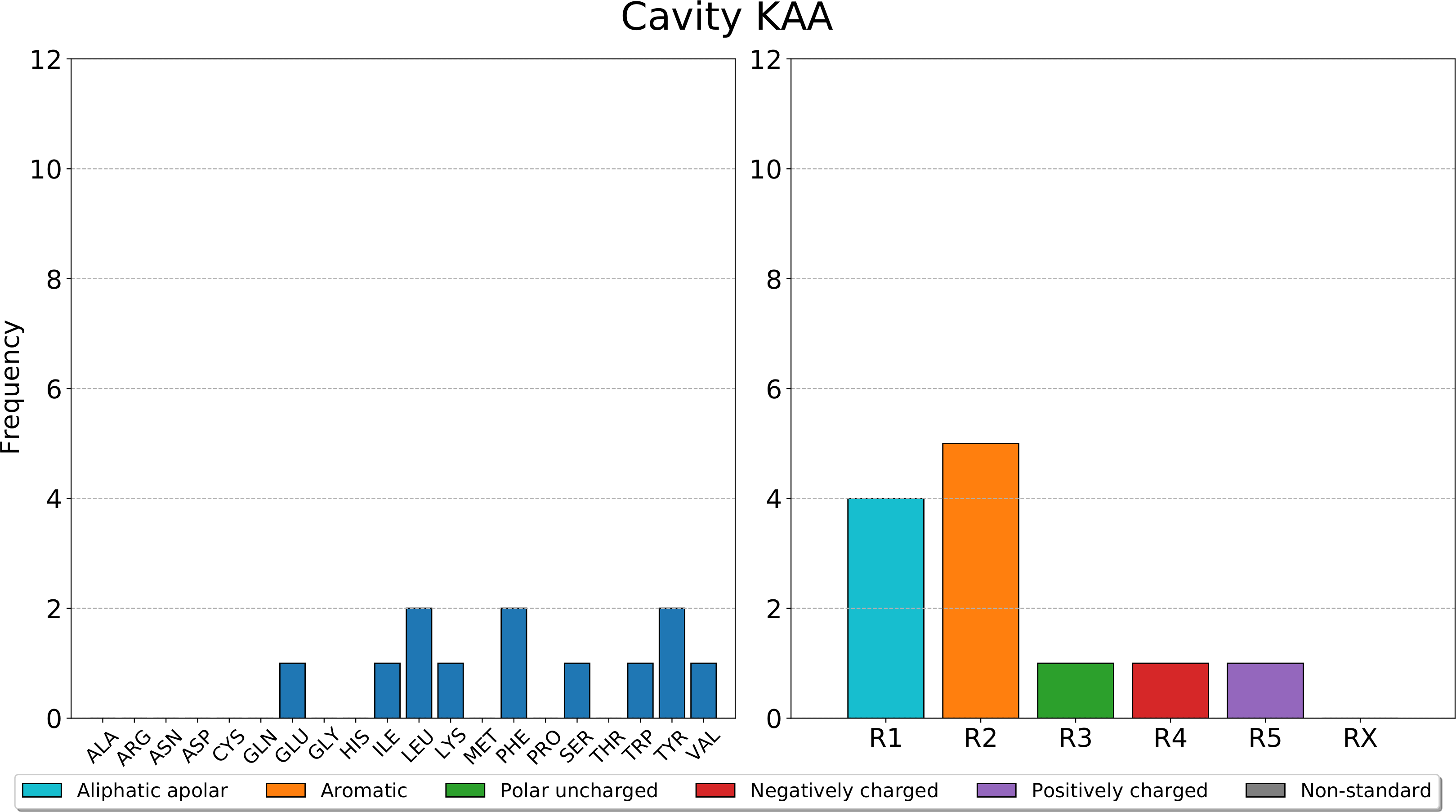
6.1 Calculating and plotting frequencies

With the interface residues defined, you can also calculate the frequencies of residues and classes of residues. The classes of residues are:

R1:: Alipathic apolar: Alanine, Glycine, Isoleucine, Leucine, Methionine, Valine
R2:: Aromatic: Phenylalanine, Tryptophan, Tyrosine
R3:: Polar uncharged: Asparagine, Cysteine, Glutamine, Proline, Serine, Threonine
R4:: Negatively charged: Aspartate, Glutamate
R5:: Positively charged: Arginine, Histidine, Lysine
RX:: Non-standard: Non-standard residues

pyKVFinder.calculate_frequencies takes the dictionary of interface residues calculated above and returns a dictionary with the frequencies of residues and classes of residues of each detected cavity.

>>> frequencies = pyKVFinder.calculate_frequencies(residues)
>>> frequencies
{'KAA': {'RESIDUES': {'GLU': 1, 'ILE': 1, 'LEU': 2, 'LYS': 1, 'PHE': 2, 'SER': 1, 'TRP': 1, 'TYR': 2, 'VAL': 1}, 'CLASS': {'R1': 4, 'R2': 5, 'R3': 1, 'R4': 1, 'R5': 1, 'RX': 0}}, 'KAB': {'RESIDUES': {'ALA': 2, 'ASN': 1, 'ASP': 1, 'LYS': 1, 'PHE': 2, 'TYR': 1, 'VAL': 1}, 'CLASS': {'R1': 3, 'R2': 3, 'R3': 1, 'R4': 1, 'R5': 1, 'RX': 0}}, 'KAC': {'RESIDUES': {'ALA': 1, 'ARG': 1, 'GLU': 1, 'HIS': 1, 'ILE': 1, 'PHE': 1, 'PRO': 2, 'THR': 2, 'VAL': 1}, 'CLASS': {'R1': 5, 'R2': 1, 'R3': 2, 'R4': 1, 'R5': 2, 'RX': 0}}, 'KAD': {'RESIDUES': {'ALA': 1, 'ASP': 1, 'GLN': 1, 'GLY': 2, 'PHE': 1, 'PRO': 1, 'TYR': 1}, 'CLASS': {'R1': 4, 'R2': 2, 'R3': 1, 'R4': 1, 'R5': 0, 'RX': 0}}, 'KAE': {'RESIDUES': {'ASN': 1, 'LEU': 3, 'LYS': 1, 'PHE': 1, 'VAL': 2}, 'CLASS': {'R1': 5, 'R2': 1, 'R3': 1, 'R4': 0, 'R5': 1, 'RX': 0}}, 'KAF': {'RESIDUES': {'ALA': 1, 'ASP': 1, 'GLN': 2, 'VAL': 1}, 'CLASS': {'R1': 2, 'R2': 0, 'R3': 2, 'R4': 1, 'R5': 0, 'RX': 0}}, 'KAG': {'RESIDUES': {'GLN': 1, 'GLU': 1, 'LEU': 1, 'PHE': 1, 'SER': 2, 'THR': 1}, 'CLASS': {'R1': 1, 'R2': 1, 'R3': 4, 'R4': 1, 'R5': 0, 'RX': 0}}, 'KAH': {'RESIDUES': {'ALA': 1, 'ARG': 1, 'ASN': 1, 'ASP': 2, 'GLN': 1, 'GLU': 4, 'GLY': 4, 'HIS': 1, 'LEU': 3, 'LYS': 2, 'MET': 1, 'PHE': 3, 'SER': 1, 'THR': 4, 'TYR': 1, 'VAL': 3}, 'CLASS': {'R1': 11, 'R2': 4, 'R3': 8, 'R4': 6, 'R5': 4, 'RX': 0}}, 'KAI': {'RESIDUES': {'HIS': 2, 'ILE': 1, 'PHE': 2, 'TYR': 1}, 'CLASS': {'R1': 1, 'R2': 3, 'R3': 0, 'R4': 0, 'R5': 2, 'RX': 0}}, 'KAJ': {'RESIDUES': {'ARG': 1, 'GLN': 1, 'GLU': 1, 'LEU': 1, 'LYS': 1, 'PHE': 1, 'PRO': 1}, 'CLASS': {'R1': 2, 'R2': 1, 'R3': 1, 'R4': 1, 'R5': 2, 'RX': 0}}, 'KAK': {'RESIDUES': {'ALA': 1, 'ILE': 1, 'LEU': 2, 'PHE': 1, 'TYR': 1}, 'CLASS': {'R1': 4, 'R2': 2, 'R3': 0, 'R4': 0, 'R5': 0, 'RX': 0}}, 'KAL': {'RESIDUES': {'ASN': 1, 'ASP': 1, 'GLU': 1, 'LEU': 1, 'PHE': 2, 'SER': 1, 'TYR': 1}, 'CLASS': {'R1': 1, 'R2': 3, 'R3': 2, 'R4': 2, 'R5': 0, 'RX': 0}}, 'KAM': {'RESIDUES': {'ARG': 2, 'ASN': 1, 'ASP': 1, 'GLY': 1, 'ILE': 2, 'LEU': 1, 'THR': 1}, 'CLASS': {'R1': 4, 'R2': 0, 'R3': 2, 'R4': 1, 'R5': 2, 'RX': 0}}, 'KAN': {'RESIDUES': {'ALA': 2, 'ARG': 1, 'ASP': 2, 'CYS': 1, 'GLY': 1, 'ILE': 1, 'LEU': 2, 'THR': 1, 'TYR': 1, 'VAL': 1}, 'CLASS': {'R1': 7, 'R2': 1, 'R3': 2, 'R4': 2, 'R5': 1, 'RX': 0}}, 'KAO': {'RESIDUES': {'ARG': 1, 'GLU': 1, 'THR': 2, 'TYR': 1}, 'CLASS': {'R1': 0, 'R2': 1, 'R3': 2, 'R4': 1, 'R5': 1, 'RX': 0}}, 'KAP': {'RESIDUES': {'GLY': 1, 'LEU': 1, 'LYS': 1, 'PHE': 1, 'TRP': 1, 'VAL': 1}, 'CLASS': {'R1': 3, 'R2': 2, 'R3': 0, 'R4': 0, 'R5': 1, 'RX': 0}}, 'KAQ': {'RESIDUES': {'GLU': 1, 'LEU': 2, 'LYS': 1, 'PRO': 1, 'VAL': 1}, 'CLASS': {'R1': 4, 'R2': 0, 'R3': 0, 'R4': 1, 'R5': 1, 'RX': 0}}, 'KAR': {'RESIDUES': {'ARG': 1, 'LYS': 2, 'PHE': 1, 'PRO': 1, 'VAL': 1}, 'CLASS': {'R1': 2, 'R2': 1, 'R3': 0, 'R4': 0, 'R5': 3, 'RX': 0}}}

Note

The cavity nomenclature is based on the integer label. The cavity marked with 2, the first integer corresponding to a cavity, is KAA, the cavity marked with 3 is KAB, the cavity marked with 4 is KAC and so on.

Afterwards, pyKVFinder.plot_frequencies takes the dictionary with the frequencies of residues and classes of residues of each detected cavity and a path to a PDF file, and plots the bar charts of calculated frequencies for each detected cavity in a PDF file.

>>> fn = 'barplots.pdf'
>>> pyKVFinder.plot_frequencies(frequencies, fn=fn)

Note

If the fn is not defined, the function automatically sets it to the default value. So, you can call the function by pyKVFinder.plot_frequencies(frequencies).

See also

A sample barplot of pyKVFinder.plot_frequencies is shown below.

7. Performing hydropathy characterization

A hydropathy characterization, that maps a target hydrophobicity scale on surface points and calculate the average hydropathy, is performed on the surface points of the detected cavities.

pyKVFinder.hydropathy takes the surface points of the detected cavities, the NumPy array with residue number, chain identifier, residue name, atom name, xyz coordinates and radius for each atom, the NumPy array with vertice coordinates (origin, X-axis, Y-axis, Z-axis), a collection of detection parameters (step, probe_in) and a target hydrophobicity scale to be mapped on the surface points, and returns a tuple with a NumPy array with the hydropobicity scale mapped to the surface points in the 3D grid and a dictionary with the average hydrophobicity scale of the detected cavities and the range of the chosen hydrophobicity scale.

>>> # Default Hydrophobicity Scale (hydropathy): 'EisenbergWeiss'
>>> hydrophobicity_scale = 'EisenbergWeiss'
>>> scales, avg_hydropathy = pyKVFinder.hydropathy(surface, atomic, vertices, step=step, probe_in=probe_in, hydrophobicity_scale=hydrophobicity_scale, ignore_backbone=ignore_backbone)
>>> scales
array([[[0., 0., 0., ..., 0., 0., 0.],
      [0., 0., 0., ..., 0., 0., 0.],
      [0., 0., 0., ..., 0., 0., 0.],
      ...,
      [0., 0., 0., ..., 0., 0., 0.],
      [0., 0., 0., ..., 0., 0., 0.],
      [0., 0., 0., ..., 0., 0., 0.]],

     ...,

     [[0., 0., 0., ..., 0., 0., 0.],
      [0., 0., 0., ..., 0., 0., 0.],
      [0., 0., 0., ..., 0., 0., 0.],
      ...,
      [0., 0., 0., ..., 0., 0., 0.],
      [0., 0., 0., ..., 0., 0., 0.],
      [0., 0., 0., ..., 0., 0., 0.]]])
>>> avg_hydropathy
{'KAA': -0.73, 'KAB': -0.05, 'KAC': -0.07, 'KAD': -0.62, 'KAE': -0.81, 'KAF': -0.14, 'KAG': -0.33, 'KAH': -0.16, 'KAI': -0.4, 'KAJ': 0.62, 'KAK': -0.99, 'KAL': 0.36, 'KAM': -0.33, 'KAN': 0.18, 'KAO': 0.88, 'KAP': -0.96, 'KAQ': 0.48, 'KAR': 0.24, 'EisenbergWeiss': [-1.42, 2.6]}

Note

The cavity nomenclature is based on the integer label. The cavity marked with 2, the first integer corresponding to a cavity, is KAA, the cavity marked with 3 is KAB, the cavity marked with 4 is KAC and so on.

Note

The pyKVFinder.hydropathy function accepts six built-in hydrophobicity scales:

EisenbergWeiss;

HessaHeijne;

KyteDoolittle;

MoonFleming;

WimleyWhite;

ZhaoLondon.

Otherwise, user must specify a .toml file following Hydrophobicity Scale File Template.

Note

If the step, probe_in, hydrophobicity_scale and ignore_backbone are not defined, the function automatically sets them to the default values. So, you can call the function by pyKVFinder.hydropathy(surface, atomic, vertices).

See also

pyKVFinder.hydropathy

8. Performing depth characterization

A depth characterization identifies the degree of burial of the binding site. First, it identifies the cavity volume boundary. Subsequently, the depth of each cavity point is heuristically estimated by the shortest Euclidean distance between the cavity point and its respective boundary points. With this, the maximum and average depths for the detected cavities are calculated.

pyKVFinder.depth takes the detected cavities and the grid spacing (step) and returns a tuple with a NumPy array with the depth of the cavity points in the 3D grid, a dictionary with the maximum depth of the detected cavities and a dictionary with the average depth of the detected cavities.

>>> depths, max_depth, avg_depth = pyKVFinder.depth(cavities, step=step)
>>> depths
array([[[0., 0., 0., ..., 0., 0., 0.],
      [0., 0., 0., ..., 0., 0., 0.],
      [0., 0., 0., ..., 0., 0., 0.],
      ...,
      [0., 0., 0., ..., 0., 0., 0.],
      [0., 0., 0., ..., 0., 0., 0.],
      [0., 0., 0., ..., 0., 0., 0.]],

     ...,

     [[0., 0., 0., ..., 0., 0., 0.],
      [0., 0., 0., ..., 0., 0., 0.],
      [0., 0., 0., ..., 0., 0., 0.],
      ...,
      [0., 0., 0., ..., 0., 0., 0.],
      [0., 0., 0., ..., 0., 0., 0.],
      [0., 0., 0., ..., 0., 0., 0.]]])
>>> max_depth
{'KAA': 3.79, 'KAB': 2.68, 'KAC': 2.62, 'KAD': 0.85, 'KAE': 3.0, 'KAF': 0.85, 'KAG': 0.6, 'KAH': 10.73, 'KAI': 0.0, 'KAJ': 2.24, 'KAK': 0.0, 'KAL': 3.0, 'KAM': 1.2, 'KAN': 0.0, 'KAO': 1.04, 'KAP': 2.08, 'KAQ': 0.85, 'KAR': 0.6}
>>> avg_depth
{'KAA': 1.35, 'KAB': 0.91, 'KAC': 0.68, 'KAD': 0.32, 'KAE': 0.99, 'KAF': 0.24, 'KAG': 0.1, 'KAH': 3.91, 'KAI': 0.0, 'KAJ': 0.96, 'KAK': 0.0, 'KAL': 1.07, 'KAM': 0.24, 'KAN': 0.0, 'KAO': 0.29, 'KAP': 0.7, 'KAQ': 0.22, 'KAR': 0.12}

Note

The cavity nomenclature is based on the integer label. The cavity marked with 2, the first integer corresponding to a cavity, is KAA, the cavity marked with 3 is KAB, the cavity marked with 4 is KAC and so on.

Note

If the step is not defined, the function automatically sets it to the default value. So, you can call the function by pyKVFinder.depth(cavities).

See also

pyKVFinder.depth

9. Exporting cavities

There are four different ways to export the detected cavities to PDB-formatted files.

9.1 Exporting only cavity points

>>> output_cavity = 'cavity_wo_surface.pdb'
>>> pyKVFinder.export(output_cavity, cavities, None, vertices, step=step)

9.2 Exporting cavity and surface points

>>> output_cavity = 'cavity.pdb'
>>> pyKVFinder.export(output_cavity, cavities, surface, vertices, step=step)

9.3 Exporting cavity and surface points with depth mapped on B-factor

>>> output_cavity = 'cavity_with_depth.pdb'
>>> pyKVFinder.export(output_cavity, cavities, surface, vertices, step=step, B=depths)

9.4 Exporting cavity and surface points with depth mapped on B-factor and hydrophobicity scale mapped on Q-factor

>>> output_cavity = 'cavity_with_depth.pdb'
>>> pyKVFinder.export(output_cavity, cavities, surface, vertices, step=step, B=depths, Q=scales)

Note

The cavity nomenclature is based on the integer label. The cavity marked with 2, the first integer corresponding to a cavity, is KAA, the cavity marked with 3 is KAB, the cavity marked with 4 is KAC and so on.

Note

If the step, B and scales are not defined, the function automatically sets them to the default values. So, you can call the function by pyKVFinder.export(output_cavity, cavities, surface, vertices).

See also

pyKVFinder.export

10. Writing results

The function call depends on the characterizations performed on the detected cavities.

10.1 Cavity detection only

>>> output_results = 'results.toml'
>>> pyKVFinder.write_results(output_results, input=pdb, ligand=None, output=output_cavity, step=step)

10.2 Spatial characterization

>>> output_results = 'results.toml'
>>> pyKVFinder.write_results(output_results, input=pdb, ligand=None, output=output_cavity, volume=volume, area=area, step=step)

10.3 Spatial and constitutional characterization

>>> output_results = 'results.toml'
>>> pyKVFinder.write_results(output_results, input=pdb, ligand=None, output=output_cavity, volume=volume, area=area, residues=residues, frequencies=frequencies, step=step)

10.4 Spatial, constitutional and depth characterization

>>> output_results = 'results.toml'
>>> pyKVFinder.write_results(output_results, input=pdb, ligand=None, output=output_cavity, volume=volume, area=area, max_depth=max_depth, avg_depth=avg_depth, residues=residues, frequencies=frequencies, step=step)

10.5 Spatial, constitutional, depth and hydropathy characterization

>>> output_results = 'results.toml'
>>> pyKVFinder.write_results(output_results, input=pdb, ligand=None, output=output_cavity, volume=volume, area=area, max_depth=max_depth, avg_depth=avg_depth, avg_hydropathy=avg_hydropathy, residues=residues, frequencies=frequencies, step=step)

Note

The cavity nomenclature is based on the integer label. The cavity marked with 2, the first integer corresponding to a cavity, is KAA, the cavity marked with 3 is KAB, the cavity marked with 4 is KAC and so on.

See also

pyKVFinder.write_results

Steered detection

All these steps showed so far were performed the detection on the whole target biomolecule; however, we can perform them on a custom 3D grid, where we can explore closed regions with a custom box, which can be defined by a .toml file.

There are three methods to define a custom 3D grid as shown in Box configuration file template.

First, we will create a box .toml file with:

Four vertices of the box (origin, X-axis, Y-axis and Z-axis):

>>> import toml
>>> fn = os.path.join(os.path.dirname(pyKVFinder.__file__), 'data', 'tests', 'custom-box.toml')
>>> box = toml.load(fn)
>>> box
{'box': {'p1': [3.11, 7.34, 1.59], 'p2': [11.51, 7.34, 1.59], 'p3': [3.11, 10.74, 1.59], 'p4': [3.11, 7.34, 6.19]}}

or

A list of residues and a padding:

>>> fn = os.path.join(os.path.dirname(pyKVFinder.__file__), 'data', 'tests', 'residues-box.toml')
>>> box = toml.load(fn)
>>> box
{'box': {'residues': [['49', 'E', 'LEU'], ['50', 'E', 'GLY'], ['51', 'E', 'THR']], 'padding': 3.5}}

A third way is to define a custom 3D grid with parKVFinder’s TOML-formatted parameters file.

>>> fn = 'box.toml'
>>> box = """
      [SETTINGS.visiblebox.p1]
      x = 3.11
      y = 7.34
      z = 1.59

      [SETTINGS.visiblebox.p2]
      x = 11.51
      y = 7.34
      z = 1.59

      [SETTINGS.visiblebox.p3]
      x = 3.11
      y = 10.74
      z = 1.59

      [SETTINGS.visiblebox.p4]
      x = 3.11
      y = 7.34
      z = 6.19
"""
>>> with open(fn, 'w') as f:
...     toml.dump(toml.loads(box), f)

Note

Users can create this box with parKVFinder PyMOL plugin (PyMOL2 parKVFinder Tools) and save the parameters file from it.

Workflows

Then, you can explore the box adjustment mode with the standard and full workflows, defining the box parameter as the filepath of one box configuration file from above (custom-box.toml, residues-box.toml or box.toml).

For instance, with custom-box.toml:

>>> pdb = os.path.join(os.path.dirname(pyKVFinder.__file__), 'data', 'tests', '1FMO.pdb')
>>> # Box configuration filepath
>>> fn = os.path.join(os.path.dirname(pyKVFinder.__file__), 'data', 'tests', 'custom-box.toml')
>>> # Standard workflow
>>> results = pyKVFinder.run_workflow(pdb, box=fn)
>>> # Full workflow
>>> results = pyKVFinder.run_workflow(pdb, box=fn, include_depth=True, include_hydropathy=True, hydrophobicity_scale='EisenbergWeiss')

See also

pyKVFinder.run_workflow

Separated steps

If you are running pyKVFinder package in a step-by-step fashion (Separated steps), the steps 3 and 4 are different than before.

Dimensioning the 3D grid: Instead of calling pyKVFinder.get_vertices, you call pyKVFinder.get_vertices_from_file.

pyKVFinder.get_vertices_from_file takes .toml file with box configuration or parKVFinder parameters file, the NumPy array with residue number, chain identifier, residue name, atom name, xyz coordinates and radius for each atom, and a collection of detection parameters (step, probe_in and probe_out), and returns a tuple with a NumPy array with vertice coordinates (origin, X-axis, Y-axis, Z-axis) of the 3D grid and the NumPy array with residue number, chain identifier, residue name, atom name, xyz coordinates and radius for each atom inside the custom box.

Users can define the box parameter as the filepath of one box configuration file from above (custom-box.toml, residues-box.toml or box.toml). For instance, with custom-box.toml:

>>> vertices, atomic = pyKVFinder.get_vertices_from_file(fn, atomic, step=step, probe_in=probe_in, probe_out=probe_out)

Note

If the step, probe_in and probe_out are not defined, the function automatically sets them to the default value. So, you can call the function by pyKVFinder.get_vertices_from_file('box.toml', atomic).

Detecting biomolecular cavities: Now, you can explore this box adjustment mode, defining the box_adjustment parameter as True.

>>> ncav, cavities = pyKVFinder.detect(atomic, vertices, step=step, probe_in=probe_in, probe_out=probe_out, removal_distance=removal_distance, volume_cutoff=volume_cutoff, box_adjustment=True, surface=surface)
>>> ncav
1
>> cavities
array([[[-1, -1, -1, ..., -1, -1, -1],
    [-1, -1, -1, ..., -1, -1, -1],
    [-1, -1, -1, ..., -1, -1, -1],
    ...,
    [-1, -1, -1, ..., -1, -1, -1],
    [-1, -1, -1, ..., -1, -1, -1],
    [-1, -1, -1, ..., -1, -1, -1]],

    ...,

    [[-1, -1, -1, ..., -1, -1, -1],
    [-1, -1, -1, ..., -1, -1, -1],
    [-1, -1, -1, ..., -1, -1, -1],
    ...,
    [-1, -1, -1, ..., -1, -1, -1],
    [-1, -1, -1, ..., -1, -1, -1],
    [-1, -1, -1, ..., -1, -1, -1]]], dtype=int32)

Note

If any of the detection parameters (step, probe_in, probe_out, removal_distance, volume_cutoff, surface) are not defined, the function automatically sets them to the default value. So, you can call the function by pyKVFinder.detect(atomic, vertices, box_adjustment=True).

Warning

If you are using box adjusment mode, do not forget to set box_adjustment flag to True.

See also

Molecular volume

All files used on this tutorial can be found in our package and in our GitHub repository:

ClO4.pdb

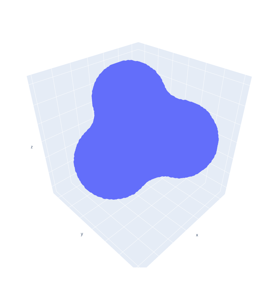
In this tutorial, we will use pyKVFinder on perchlorate (ClO₄ ) to estimate the molecular volume, using van der Waals (vdW) surface, solvent excluded surface (SES) and solvent accessible surface (SAS) to represent the molecular surface (see Figure below).

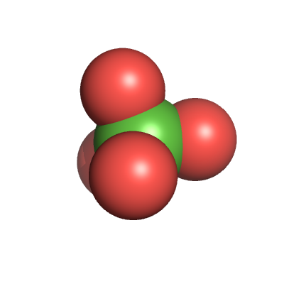
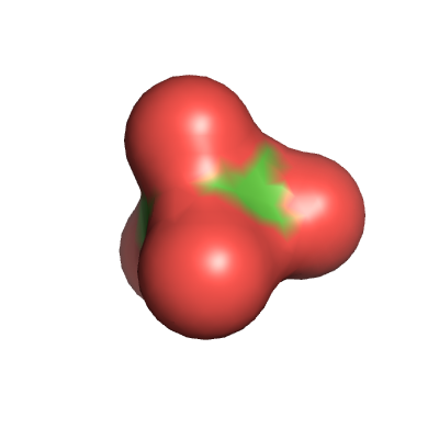
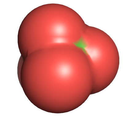
(a) vdW	(b) SES	(c) SAS
Molecular surface represenation

First, we must load the target molecular structure (ClO₄ ) into pyKVFinder.Molecule class.

>>> pdb = os.path.join(os.path.dirname(pyKVFinder.__file__), 'data', 'tests', 'ClO4.pdb')
>>> molecule pyKVFinder.Molecule(pdb)
>>> molecule
<pyKVFinder.main.Molecule object at 0x7f5ddacf2230>

With the atomic information and vdW radii dictionary loaded, the molecule is inserted into a regular 3D grid, considering the vdW radii of any of the atoms. Natively, the vdW radii are taken from the built-in dictionary. In the 3D grid, each voxel corresponds to a molecule (0) or solvent (1) points. Here, we can model our molecule using the vdW surface, SES or SAS.

1. vdW volume

Molecule.vdw() takes a grid spacing and returns a NumPy array with the molecule points representing the vdW surface in the 3D grid.

>>> # Grid Spacing (step): 0.1
>>> step = 0.1
>>> molecule.vdw(step=step)
>>> molecule.grid
array([[[1, 1, 1, ..., 1, 1, 1],
        [1, 1, 1, ..., 1, 1, 1],
        [1, 1, 1, ..., 1, 1, 1],
        ...,
        [1, 1, 1, ..., 1, 1, 1],
        [1, 1, 1, ..., 1, 1, 1],
        [1, 1, 1, ..., 1, 1, 1]],

        ...,

      [[1, 1, 1, ..., 1, 1, 1],
        [1, 1, 1, ..., 1, 1, 1],
        [1, 1, 1, ..., 1, 1, 1],
        ...,
        [1, 1, 1, ..., 1, 1, 1],
        [1, 1, 1, ..., 1, 1, 1],
        [1, 1, 1, ..., 1, 1, 1]]], dtype=int32)

Note

If step is not defined, the function automatically sets it to the default value. So, you can call the function by molecule.vdw().

We can preview our modelled molecule in the 3D grid by running:

>>> molecule.export("vdw-model.pdb")

We can also export our modelled molecule int the 3D grid by running:

>>> molecule.preview()

Now, we can estimate the vdW volume by running:

>>> molecule.volume()
83.64

2. SES volume

Molecule.surface() takes the grid spacing, the spherical probe size to model the surface, the SES representation and returns a NumPy array with the molecule points representing the SES in the 3D grid.

>>> # Grid Spacing (step): 0.1
>>> step = 0.1
>>> # Spherical Probe (probe): 1.4
>>> probe = 1.4
>>> # Surface Representation: SES
>>> surface = 'SES'
>>> molecule.surface(step=step, probe=probe, surface=surface)
>>> molecule.grid
array([[[1, 1, 1, ..., 1, 1, 1],
        [1, 1, 1, ..., 1, 1, 1],
        [1, 1, 1, ..., 1, 1, 1],
        ...,
        [1, 1, 1, ..., 1, 1, 1],
        [1, 1, 1, ..., 1, 1, 1],
        [1, 1, 1, ..., 1, 1, 1]],

        ...,

      [[1, 1, 1, ..., 1, 1, 1],
        [1, 1, 1, ..., 1, 1, 1],
        [1, 1, 1, ..., 1, 1, 1],
        ...,
        [1, 1, 1, ..., 1, 1, 1],
        [1, 1, 1, ..., 1, 1, 1],
        [1, 1, 1, ..., 1, 1, 1]]], dtype=int32)

Note

If any of the parameters (step, probe or surface) are not defined, the function automatically sets them to the default values. So, you can call the function by molecule.surface().

We can preview our modelled molecule in the 3D grid by running:

>>> molecule.preview()

Now, we can estimate the vdW volume by running:

>>> molecule.volume()
90.8

3. SAS volume

Molecule.surface() takes a grid spacing, a spherical probe to model the surface, a SAS representation and returns a NumPy array with the molecule points representing the SES in the 3D grid.

>>> # Grid Spacing (step): 0.1
>>> step = 0.1
>>> # Spherical Probe (probe): 1.4
>>> probe = 1.4
>>> # Surface Representation: SAS
>>> surface = 'SAS'
>>> molecule.surface(step=step, probe=probe, surface=surface)
>>> molecule.grid
array([[[1, 1, 1, ..., 1, 1, 1],
        [1, 1, 1, ..., 1, 1, 1],
        [1, 1, 1, ..., 1, 1, 1],
        ...,
        [1, 1, 1, ..., 1, 1, 1],
        [1, 1, 1, ..., 1, 1, 1],
        [1, 1, 1, ..., 1, 1, 1]],

        ...,

      [[1, 1, 1, ..., 1, 1, 1],
        [1, 1, 1, ..., 1, 1, 1],
        [1, 1, 1, ..., 1, 1, 1],
        ...,
        [1, 1, 1, ..., 1, 1, 1],
        [1, 1, 1, ..., 1, 1, 1],
        [1, 1, 1, ..., 1, 1, 1]]], dtype=int32)

Note

If any of the parameters (step or probe) are not defined, the function automatically sets them to the default values. So, you can call the function by molecule.surface(surface='SAS').

We can preview our modelled molecule in the 3D grid by running:

>>> molecule.preview()

Now, we can estimate the vdW volume by running:

>>> molecule.volume()
340.28

Examples

Jupyter notebook examples are available for: